Introducing the latest article in our Data Deep Dive series, image-to-text: latent diffusion models
Written by NICD Data Scientists Dr Antonia Kontaratou and Louise Braithwaite MSc
Introduction to text-to-image models
Text-to-image models are artificial intelligence systems that generate images from text descriptions. They are classified as generative models and form a sub-field of Deep Learning, which utilises artificial neural networks to learn representations of data. Generative models have gained significant attention, through the release of consumer AI tools such as ChatGPT for text generation, GitHub Copilot for code generation and DreamStudio for image generation. They have the remarkable ability to create novel new forms of media resembling the patterns they learnt from the data they are trained on. In addition to the three modalities mentioned above, generative models are being developed for other modalities including audio and video.
If you wish to explore text-to-image tools there are a number of paid for and free platforms where you can explore the abilities of these models. Some examples include:
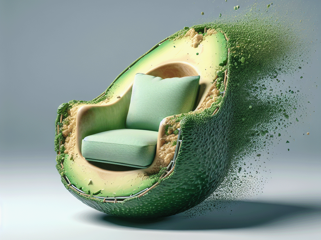
The image of the avocado armchair at the top of the page is an example of an image generated from a prompt using DALL·E. To generate this image the prompt, "3D render an avocado style armchair diffusing into latent space" was used.
Whilst, these models and their commercial counterparts are still in their infancy they have been adopted by both enthusiasts and professionals. Within the creative industries these tools support tasks such as content creation and product development by enabling professionals to easily generate, edit and modify images through text prompts. If you are interested in learning more about the capabilities of these models OpenAI provide a research publication evaluating the capabilities their text-to-image model, DALL·E.
Image generation models can be categorised into three main types: variational autoencoders, adversarial models and latent diffusion models. This blog will focus on latent diffusion models. We will explore:
-
the different components of these models,
-
how they are trained,
-
the image generation mechanisms they use,
-
how they integrate textual information,
-
and present how the final image output is influenced by text prompts.
Introduction to latent diffusion models
Latent diffusion models for image generation became popular in 2022 in the paper High-Resolution Image Synthesis with Latent Diffusion Models by Rombach et al that presented a novel approach to image synthesis.

Figure 1: Overview of the latent diffusion model; left: high level overview, right: detailed presentation of components from the Rombach et al paper
Figure 1 presents the system proposed by the authors, the components of which we will try to unveil in the following sections. A simplified overview of this diagram is presented alongside the original and it consists of three main parts: the pixel space, latent space and text.
The pixel space is where images are processed into a lower-dimensional representation before being passed to the model and then back into an image after the diffusion process has occurred (covered in section 1). The text part is where text is processed prior to being passed to the model (covered in section 5). The latent space is where the diffusion process happens. In this space the model no longer works with the original images, but rather with "smaller representations" (covered in sections 2, 3 and 4). These three components are comprised of different processing steps and models that enable the text-to-image generation: pixel space uses an autoencoder model, latent space utilises a diffusion process and denoising U-Net model and text uses a CLIP tokeniser model.
Let's have a closer look at all these parts.
Section 1: pixel space
At this point it would be good to remind ourselves of how images are stored in computers. Grayscale images are stored as a grid of pixels, where each pixel's value ranges between 0 and 255 and represents the brightness level of that particular point in the image, with 0 being black and 255 white. Coloured images are stored similarly, but with three colour channels: red, green, and blue (RGB). Each value in each channel contains information about the pixel's colour level ranging again between 0 and 255. Combinations of these values create the full colour palette. So, if a coloured image has a resolution of 1920x1080 pixels (Full HD) then it has the dimensions 3x1920x1080 (3 channels RGB, width, height) in the pixel space.
Figure 2: Autoencoder model that creates lower-dimensional image embeddings and reconstructs the image
Deep learning models utilise lower-dimensional representations, known as embeddings, of images to reduce computation and gain a holistic understanding of the images' features. These embeddings, which encode essential aspects of the original input images, form what is referred to as the latent space.
An example of such a model is the autoencoder, which effectively generates these representations and compresses the initial information. It consists of two parts, an encoder (ℰ) and a decoder (𝒟). The encoder creates the low-dimensional representations and the decoder reconstructs the original dimensions. The loss function, that captures and informs the model how well it performs at its task, quantifies the difference between the input and the reconstructed image from the latent space representation. Through training on diverse images, the autoencoder learns to generate high-quality lower-dimensional representations that capture well the information presented in the original image. Subsequently, the decoder is able to project a latent representation to the original dimensions.
After using the encoder to extract low-dimensional embeddings from the input images, the latent diffusion models work with these embeddings.
With this, we have completed the first step of understanding the diffusion process! We are now working at the latent space!
Section 2: latent space
Moving on to the operations happening in the latent space, in this section we will focus only on the image part and we will not incorporate any information from the prompt yet. The task of generating images with no condition in any context (e.g. a text prompt or another image) is called unconditional image generation.
But first, let's clarify the difference between training and inference. In deep learning we want to perform a specific task such as image classification, text summarisation or, as in our case, image generation, using a model (which can also be thought of as a very large and complex mathematical function). During training, a model accepts numerous example data, such as images, as input with the aim to improve its performance on the specific task by adjusting its parameters through repeated iterations to minimise errors. In supervised learning as opposed to unsupervised learning, input data must also contain ground truth labels. For example, for image classification we have to provide the actual class the image depicts e.g. cat, flamingo, pedestrian etc. Once the model is trained, it can be used for inference, where it will apply its learned knowledge to make predictions or perform tasks on unseen data. During inference, a model does not adjust its parameters anymore, it uses its learned patterns to real-world scenarios.
So, in the sections that follow, let's focus on the "green" part of our initial diagram (Figure 1) and try to present the components of the latent diffusion models that work with images in the latent space. In the following figure (Figure 3) we have isolated this part.
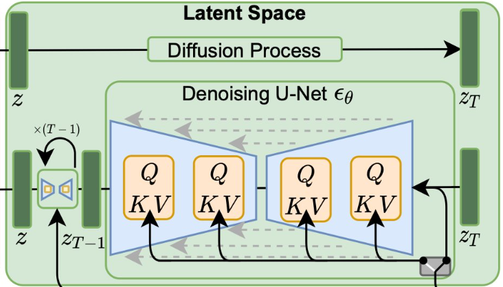
Figure 3: Components of the latent diffusion models that operate in the latent space
Section 3: Training a latent diffusion model
You will soon notice that a term frequently used in the context of latent diffusion models is 'noise'. It is usually Gaussian noise, a type of noise with Gaussian distribution (with mean of 0 and variance of 1) and it can be considered as random variations in pixel values that do not correspond to the underlying scene being captured.
As mentioned earlier, we are now operating in the latent space, which means that each original image is now transformed into a lower-dimension representation. However, for explanatory purposes we will use examples with the original images to demonstrate the process.
For supervised learning we need a lot of input examples to train a model. Specifically for training latent diffusion models, we have a lot of input images on which we add controlled noise at various timesteps (Figure 4). This process is known as forward diffusion.
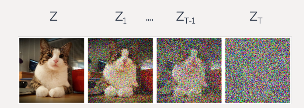
Figure 4: Forward diffusion process. Source: Nvidia blog
Then, we use samples from these noisy images at random timesteps along with their ground truth added noise as inputs to train our model. The model aims to predict the noise present in a given image. Initially, it generates random predictions but over time it refines them by adjusting its parameters based on the calculated loss which compares the predicted noise to the ground truth. After several rounds of training, the model is now able to predict noise and predict a ‘noisy image’ embedding 𝑧T-1 (at timestamp T-1) having started from a ‘noisy image’ embedding (𝑧T at timestamp T). This is called the *denoising process* also referred to as *reverse diffusion process* (Figure 5).
The neural network used in the denoising process is a U-Net, a convolutional neural network (CNN) U-shaped architecture. Originally, this model was used for computer vision and image segmentation tasks but over the last years it has also been used for image restoration and noise prediction which is of our interest. It consists of an encoder that downsamples and extracts features from the input image (in our case 'noisy image' embeddings), and a decoder which upsamples intermediate features to produce the final output (in our case the predicted noise).
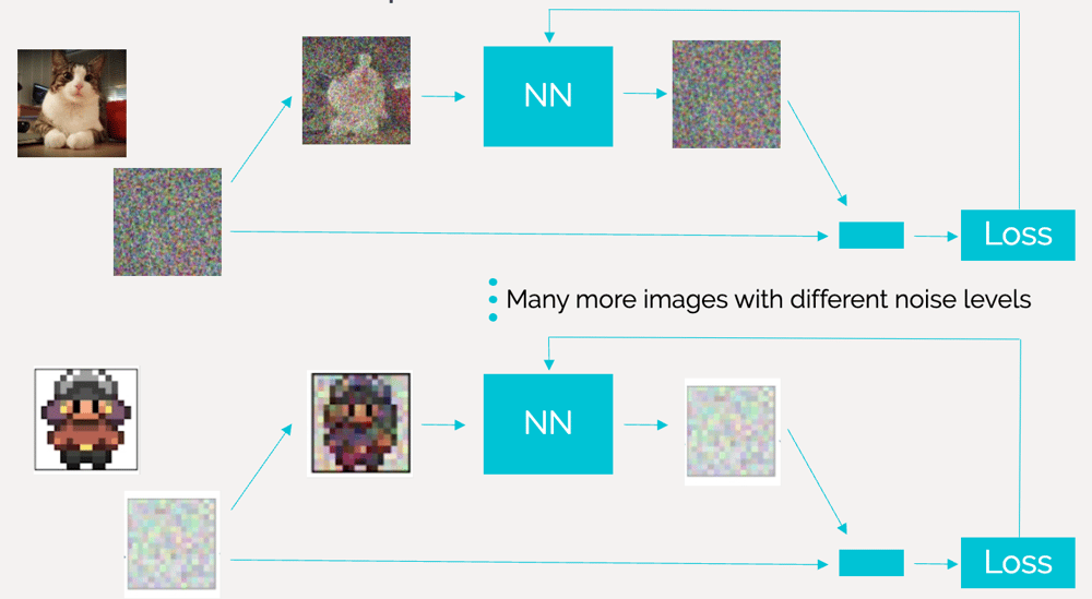
Figure 5: Training latent diffusion models. Source: DeepLearning.AI
Once trained, the model can be used for generating an image which will contain characteristics based on the features and patterns it has learned during training. The image generation process is also known as 'sampling'.
Section 4: sampling
During sampling, the trained model typically starts with a random latent vector sampled from a simple distribution, such as Gaussian, and it is usually nothing more but pure noise. Then, it applies the diffusion process in reverse, gradually reducing the noise level in the latent space representation to generate high-quality images. As shown in Figure 6, the sampling process requires numerous iterations because each iteration corresponds to a step in the reverse diffusion process that performs a level of noise reduction. The number of iterations required can vary due to different factors such as the complexity of the model architecture and the desired level of image quality. Hence, it is usually determined through experimentation.
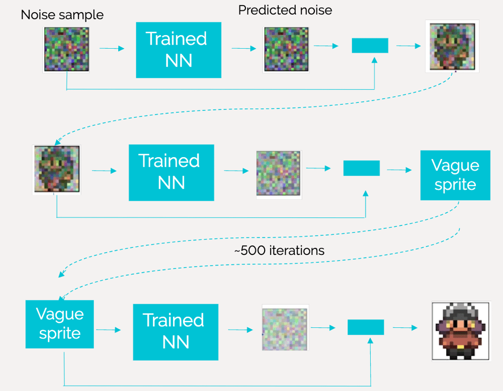
Figure 6: Image generation - sampling. Source: DeepLearning.AI
You might be wondering whether a trained model produces a different output every time the generation process is applied and the required iterations completed. The answer is yes. There is inherent randomness in the process, therefore small variations in the latent vectors can lead to different outputs each time the model is sampled.
The last stage involves converting the output latent representation into a tangible image. Recall how we initially transitioned from the pixel space to the latent space using the encoder? It's likely no surprise that we'll now reverse the process, going from the latent representation to an actual image using the decoder! Hopefully, the image is realistic and visually appealing!
Section 5: text
We'll now outline the process of processing text before feeding it into the denoising U-Net model. Text is inputted into the model in two ways: first, during the model's training phase with image-text pairs; and second, after the model is trained, as a prompt to guide the subject and style of the generated image.
This section will explore two key elements:
1. working with text - turning text into text embeddings
2. CLIP - the multimodal model used to create text embeddings that are passed to the latent space
Working with text
Natural language processing (NLP) is a subfield of artificial intelligence (AI) concerned with developing systems that deal with processing, understanding and generating natural language. Text representation is a key part of NLP and is focused on developing methods for converting text data into machine-readable form whilst maintaining the complex features of written language. These representations are referred to as text embeddings.
The growth of AI consumer tools, such as ChatGPT, demonstrate the increased capabilities of state of the art language models. Commonly referred to as large language models (LLMs), this term characterises models that are trained on vast amounts of text data and can comprehend and generate human language text. They are enabled by transformer based architectures and self-supervised learning techniques. If you are interested in learning more about LLMs the 'What are Large Language Models?' resource hosted by Cohere is a good starting point.
Pre-trained LLMs can be used to generate text embeddings. A mechanism known as attention enables these models to capture the complexity of language by updating the text embeddings to reflect the context of the text input. This means that words that have different meanings in different contexts are more accurately represented in the generated text embeddings. For example, the word "bat" can refer to a piece of sports equipment or a type of flying mammal. As a human you are able to comprehend the correct meaning based upon the context the word is used. The attention mechanism enables the embedding to update based upon the context too.
Figure 7 shows that text embeddings that are numerically similar are also semantically similar. For example, the embedding vector of “canine companions say” will be more similar to the embedding vector of “woof” than of “meow”.
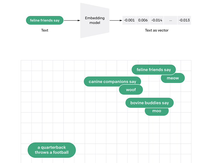
Figure 7: Taken from an OpenAI blog, the figure shows how text can be passed to an embedding model to generate a list of numbers (vector). The plot demonstrates that the generated embeddings that are numerically similar are also semantically similar. For example, the embedding vector of “canine companions say” will be more similar to the embedding vector of “woof” than of “meow”.
CLIP
Stable Diffusion is an example of a latent diffusion model, which was trained on a large-scale dataset called LAION-5B. LAION-5B contains 5.85 billion image-text pairs collected from the internet by an organisation called Common Crawl. The text is extracted from the alt-text attribute of HTML IMG tags, which means they should contain more information about the image than a classic classification label, such as "dog", "cat", "car", "building" etc.
The powerful pre-trained language models discussed in the previous section could be used to process the alt-text attributes into text embeddings but this is no longer common practice. Instead of using a LLM to generate text embeddings a multimodal model, such as CLIP is used. Multimodal models integrate text and image data into a shared embedding space, which results in enhanced understanding and performance across various tasks.
Contrastive Language-Image Pretraining (CLIP), is a deep learning model first developed by OpenAI in 2021. CLIP brings text and image representations into the same embedding space, enabling direct comparisons between the two modalities. Stable Diffusion uses a variation of this model, Open CLIP, to generate the text embeddings that will be passed to the U-Net.
CLIP is able to merge the image and text embedding spaces by training the model to bring related image-text pairs closer together while pushing unrelated ones apart. It accomplishes this by utilising a contrastive training objective. This means the model is contrasting what we know goes together, an image and its text caption, with what we know doesn't go together, other text captions and images in the batch. This approach creates a classification task, where we want a high score for the image-text pairs and low scores for the non-matches (Figure 8).
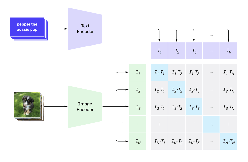
Figure 8: taken from the OpenAI CLIP blog, the figure shows how the model will aim to generate a high scores for the correct image-text pairs and low scores for the non-matches.
Image-text pairs are more likely to contain more text information than a short classification label, such as "dog", "cat", "hamster" etc. As the model is exposed to larger datasets it is able to learn much more. For example, it would not just learn to identify food, it would also be able to identify different cuisines, dishes and ingredients.
The core benefit of using a multimodal model to create a "text" embedding is that it generates a joint image-text representation. Not only do these embeddings contain a semantic and syntactic understanding of text they also understand image information such as visual features e.g., shapes, colours and textures, detection of objects within the image and the spatial relationships between objects. It is the additional information, held in the multimodal embeddings that provide the model with the capability to generate images that reflect complex visual descriptions.
Section 6: joining all the parts
This blog has identified that a latent diffusion model consists of three core models, an autoencoder, a denoising U-Net and a model to encode the conditioning information, such as CLIP.
Autoencoders transform an image from pixel space to latent space by creating embeddings, and vice versa. The diffusion process creates the noisy image embeddings needed to train the model. The denoising U-Net learns to predict the noise in the image embeddings. Finally, a CLIP model is used to create rich embeddings that bring together text and image modalities. So far, we've explored the training process of these models and sampling without text prompts. Now, it's time to connect these pieces together and explore how we can generate images from text. Let's revisit the diagram of the latent diffusion model from the original paper (Figure 9) and see how training and sampling are possible.
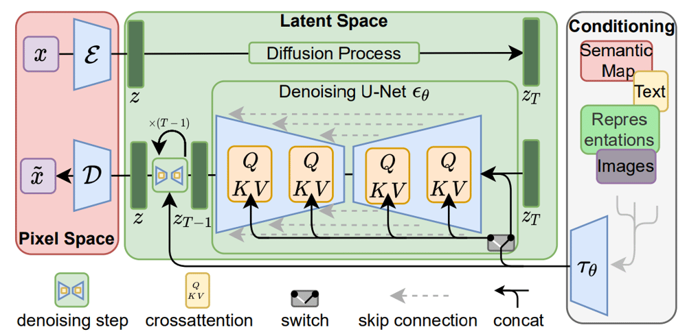
Figure 9: Latent diffusion model, High-Resolution Image Synthesis with Latent Diffusion Models, Rombach et al, 2022
Section 7: training
In section 3 we saw how we can train latent diffusion models to create images without providing an accompanying text (Figure 5). To train the model to be able to combine information from both images and text we have to follow a similar process (using forward diffusion and denoising), however now we not only provide training images but also a text associated with it. For example, looking in Figure 11, we can see that we provide the model with an image embedding and a text embedding. After passing many examples of image-text pairs to the model it will learn to associate the text with patterns in the images.
To integrate the text embedding into the latent space a mechanism called cross-attention is applied. Cross attention uses matrix multiplication to combine information from two modalities. Importantly, it also allows the model to relate relevant words in the text to the corresponding regions in the image.
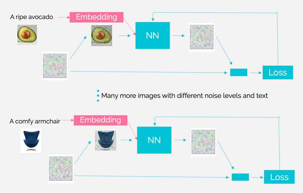
Figure 10: Training latent diffusion models using images and text. Source: DeepLearning.AI
Section 8: sampling
During sampling, as before, the model has to generate an image starting from a sample of random noise, however now it must condition the image generation to the prompt provided (Figure 11). The cross-attention mechanism allows the model to attend to relevant parts of the input image and text simultaneously, aligning features across modalities to facilitate coherent and contextually relevant image generation.

Figure 11: Image generation - sampling using prompt
The trained model is then able to generate images from notions related to images and text it has learned during training. So, if it has been trained on associating the words "avocado" and "armchair" with specific image patterns, it should be able to generate an image of the famous "avocado armchair" (Figure 12)!
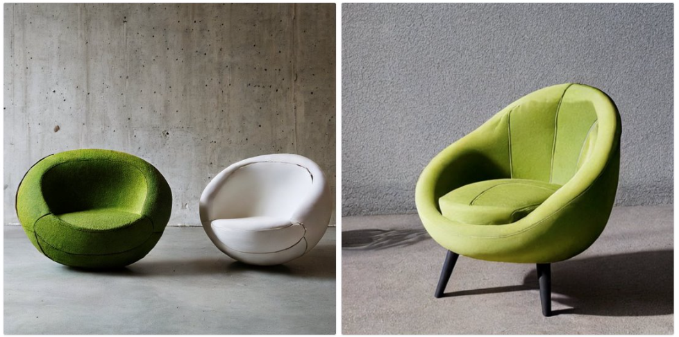
Figure 12: An avocado armchair. Image generated using Stable Diffusion - Hugging Face
Conclusion
In summary, through this blog we uncovered some core ideas behind the workings of text-to-image models, examining how they generate visual content from textual prompts. We explored the mechanisms of latent diffusion models and the role of CLIP in enabling cross-modal comprehension. We also discussed how image generation can be conditioned on text to create visual outputs that are guided by textual prompts.
With these insights, you should now have a better understanding of the underlying technical intricacies every time that you use image Generative AI to craft artistic images from prompts!
Read more technical blogs from our expert Data Scientists.
