
This blog post aims to introduce the various R packages making up the tidymodels metapackage by classifying Iris flower species from the Iris dataset. The Iris dataset is so famous it has its own Wikipedia Page. It consists of measurements of sepal and petal lengths and widths and the corresponding species name. A traditional machine learning task is to identify the species from the other measurements.
The current workflow for a typical classification (or regression) model in tidymodels is:
- Split the data into training and test sets
- Define pre-processing steps using recipes
- Create a model using parsnip
- Combine the model and recipe into a workflow
- Perform hyper-parameter tuning using cross validation on the training data using tune
- Select the hyper-parameters which minimise (or maximise) a selected metric using cross validation on the training data
- Fit the selected model to the training data
- Evaluate the model on the test set
It is worth noting that tidymodels is in active development and hence the user facing API is not stable.
To begin, we load in the Iris data. The data is available in the datasets R package which comes with a base installation of R and so can be loaded using the data function.
data(iris)
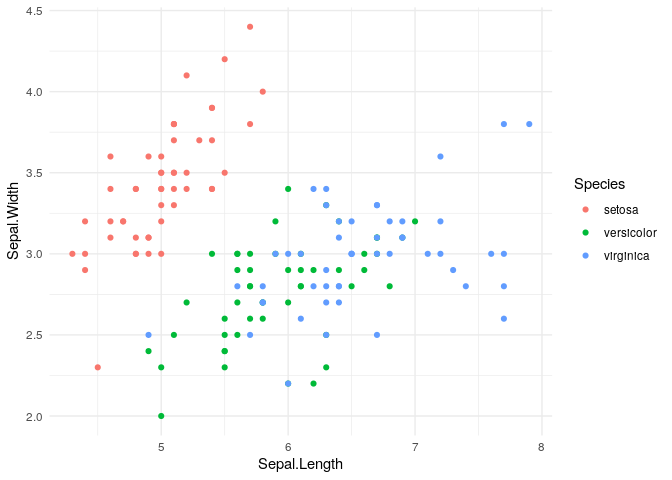
Typically we would explore the data before beginning modelling. We can produce a plot of the Iris data.
iris %>%
      ggplot(aes(x = Sepal.Length, y = Sepal.Width, colour = Species)) +
      geom_point()
Now, split the iris data into training and test sets. We use initial_split to perform stratified sampling using the outcome variable Species. Stratified sampling ensures that there are examples of each class in our test set and training set. The parameter prop specifies the proportion of data used to create the training set. We have chosen prop to be 4/5, meaning that we keep approximately 80% (= 4/5) of the data for training and 20% of the data for the testing set. The purpose of splitting the data into training and testing sets is to avoid over-fitting and allow us to understand how our chosen model will perform on new, unseen data. For that reason, the test set is not used in selecting the model or model hyper-parameter tuning.
set.seed(1) # Set a seed to get reproducible splits
split <- rsample::initial_split(iris, strata = Species, prop = 4/5)
train <- rsample::training(split)
test <- rsample::testing(split)
Next a recipe is used to pre-process the data. In the Iris dataset there is no missing data. However we could specify imputation techniques here or choose to omit examples with missing values. We decide to centre and scale the predictors. This will help when fitting a regression model since all the predictors will be on the same scale resulting in a stable design matrix.
rec <- recipe(Species ~ ., data = train) %>%
      step_center(all_predictors()) %>%
      step_scale(all_predictors())
Next we specify a multinomial regression model using the engine glmnet. glmnet is an R package for fitting generalised linear models using an elastic net penalty. The elastic net penalty is a combination of lasso, or L1 regularisation (for feature selection) and ridge, or L2 regularisation (for coefficient shrinking). We leave the penalty and mixture arguments unspecified and instead using the function tune(). This means we can learn these hyper-parameters by minimising a performance metric (such as accuracy) using \(k\)-fold cross validation on the training set.
model <- multinom_reg() %>%
      set_engine("glmnet") %>%
      set_args(penalty = tune(), mixture = tune())
The recipe and model can be combined together into a workflow.
wf <- workflow() %>%
      add_recipe(rec) %>%
      add_model(model)
Next, create a \(k\)-fold cross validation dataset using training data. This creates 10 random splits of the data which can be used to perform hyper-parameter optimisation.
cv <- rsample::vfold_cv(train, strata = Species, v = 10)
Use grid search to find some good hyper-parameters. This evaluates different values of penalty and mixture for each of the folds and records the ROC-AUC and accuracy metrics for each model. Grid search becomes inefficient when then number of hyper-parameters becomes large and more sophisticated optimisation algorithms can be used.
hyper_parameters <- tune::tune_grid(wf, resamples = cv)
We can view the metrics for a selection of the hyper-parameters.
collect_metrics(hyper_parameters)
| penalty | mixture | .metric | .estimator | mean | n | std_err |
|---|---|---|---|---|---|---|
| 0.00 | 0.98 | accuracy | multiclass | 0.97 | 10 | 0.01 |
| 0.00 | 0.98 | roc_auc | hand_till | 1.00 | 10 | 0.00 |
| 0.00 | 0.69 | accuracy | multiclass | 0.96 | 10 | 0.02 |
| 0.00 | 0.69 | roc_auc | hand_till | 1.00 | 10 | 0.00 |
| 0.00 | 0.52 | accuracy | multiclass | 0.96 | 10 | 0.02 |
| 0.00 | 0.52 | roc_auc | hand_till | 1.00 | 10 | 0.00 |
| 0.00 | 0.81 | accuracy | multiclass | 0.98 | 10 | 0.01 |
| 0.00 | 0.81 | roc_auc | hand_till | 1.00 | 10 | 0.00 |
| 0.00 | 0.11 | accuracy | multiclass | 0.98 | 10 | 0.02 |
| 0.00 | 0.11 | roc_auc | hand_till | 1.00 | 10 | 0.00 |
| 0.00 | 0.21 | accuracy | multiclass | 0.98 | 10 | 0.02 |
| 0.00 | 0.21 | roc_auc | hand_till | 1.00 | 10 | 0.00 |
| 0.00 | 0.49 | accuracy | multiclass | 0.98 | 10 | 0.02 |
| 0.00 | 0.49 | roc_auc | hand_till | 1.00 | 10 | 0.00 |
| 0.00 | 0.02 | accuracy | multiclass | 0.98 | 10 | 0.02 |
| 0.00 | 0.02 | roc_auc | hand_till | 1.00 | 10 | 0.00 |
| 0.01 | 0.79 | accuracy | multiclass | 0.96 | 10 | 0.02 |
| 0.01 | 0.79 | roc_auc | hand_till | 1.00 | 10 | 0.00 |
| 0.40 | 0.36 | accuracy | multiclass | 0.86 | 10 | 0.03 |
| 0.40 | 0.36 | roc_auc | hand_till | 0.96 | 10 | 0.01 |
Use select_best to select the hyper-parameters which correspond to the highest value of ROC AUC.
best_hp <- select_best(hyper_parameters, metric = "roc_auc")
We can use the function tune::finalized_workflow to select the best performing workflow using the selected hyper-parameters best_hp.
best_workflow <- tune::finalize_workflow(wf, best_hp)
We can now determine the performance of the algorithm using a selection of metrics, we choose accuracy, precision and f1-measure. The test set performance is indicative of what we can expect on unseen iris examples. We fit on the entire training set using tune::last_fit, the first argument to the function is the best workflow selected using finalized_workflow, we also provide the split used to split the initial dataset into training and testing datasets and the set of metrics, metrics. The metric collection is specified using functions from yardstick.
metrics <- metric_set(accuracy, precision, f_meas)
    final_fit <- last_fit(object = best_workflow, split = split, metrics = metrics)
We can see the performance on the test-set using collect_metrics
collect_metrics(final_fit)
| .metric | .estimator | .estimate |
|---|---|---|
| accuracy | multiclass | 0.93 |
| precision | macro | 0.93 |
| f_meas | macro | 0.93 |
Finally, we fit the model to the full dataset to use for classifying future observations of Iris flowers.
best_model <- extract_model(fit(best_workflow, iris))